20 Code
There are many ways to render and compile code using Bookdown. Here are most of the “language engines” (programming languages) available to render, run and compile in Bookdown.
##  [1] "awk"         "bash"        "coffee"      "gawk"        "groovy"
##  [6] "haskell"     "lein"        "mysql"       "node"        "octave"
## [11] "perl"        "php"         "psql"        "Rscript"     "ruby"
## [16] "sas"         "scala"       "sed"         "sh"          "stata"
## [21] "zsh"         "asis"        "asy"         "block"       "block2"
## [26] "bslib"       "c"           "cat"         "cc"          "comment"
## [31] "css"         "ditaa"       "dot"         "embed"       "eviews"
## [36] "exec"        "fortran"     "fortran95"   "go"          "highlight"
## [41] "js"          "julia"       "python"      "R"           "Rcpp"
## [46] "sass"        "scss"        "sql"         "stan"        "targets"
## [51] "tikz"        "verbatim"    "theorem"     "lemma"       "corollary"
## [56] "proposition" "conjecture"  "definition"  "example"     "exercise"
## [61] "hypothesis"  "proof"       "remark"      "solution"    "glue"
## [66] "glue_sql"    "gluesql"
20.1 Rendering Code
Just rendering code refers to Bookdown formatting code so that our users can view it. The code does not run or compile. An example is shown below.
```
insert code here
```
which appears as
insert code hereThese are called “code chunks”.
20.2 Syntax highlighting
Bookdown has syntax highlighting for the languages shown above. To implement this, add the name of the language after the first 3 ` symbols. Note that the language is not case sensitive (so both “r” and “R” would render the same below). For example:
```r
x <- 42
x
```
renders into:
Notice that since <- is how to assign values to variables in R, it is highlighted. If we were to replace “r” with a different language, this may not be highlighted (depending if “<-” is a relevant symbol in that language.)
20.3 Running code
To have the code actually compile, we need to put “{” and “}” brackets around the language. For example:
```{r}
x <- 42
x
```renders and compiles into:
## [1] 42The second bar you see is the output of the R commands. This can be used to create and display images and charts.
```{r fig, out.width='80%', fig.asp=.75, fig.align='center', fig.alt='Plot with connected points showing that vapor pressure of mercury increases exponentially as temperature increases.'}
par(mar = c(4, 4, .1, .1))
plot(pressure, type = 'b', pch = 19)
```
renders and compiles into:

You can run these “code chunks” without previewing or building the book. To the right of your code chunk, there are 3 symbols (as seen below).
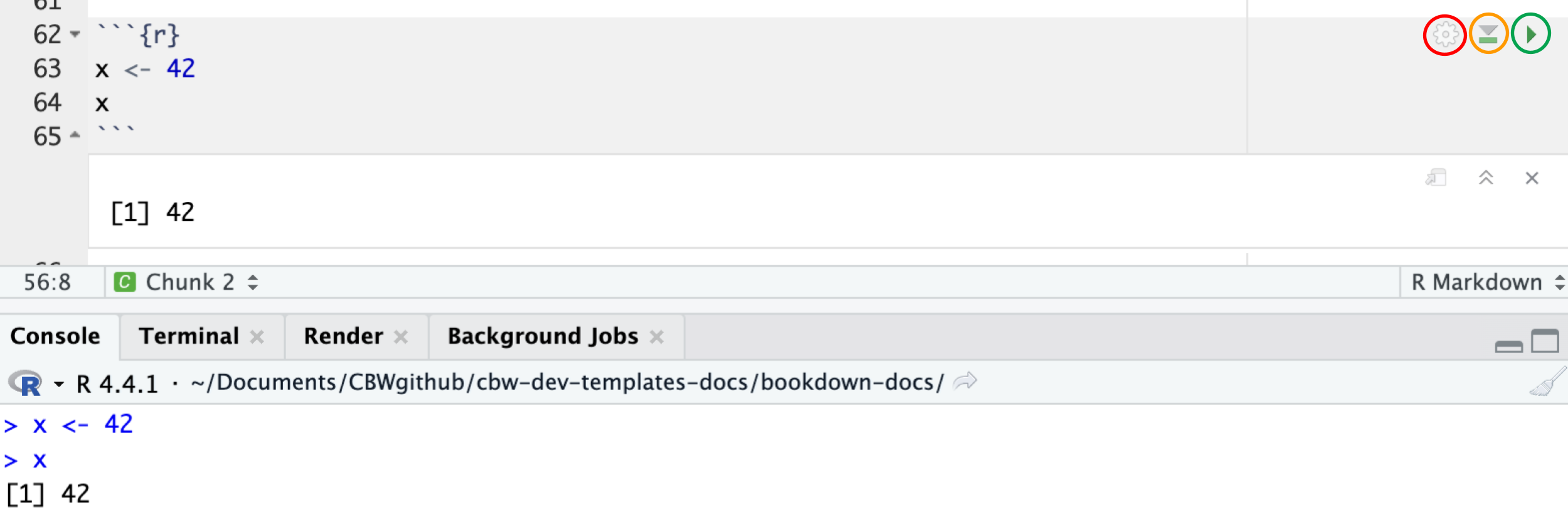
The gear symbol opens chunk options.
The down arrow symbol runs all previous chunks and the current chunk. This is helpful if previous chunks define a variable that you will need in your current chunk.
Note: This means we can use variables from previous chunks.
The right-pointing arrow symbol runs the current code chunk. A rectangular box will appear below your code chunk, with the output of your code.
Additionally, notice that in your bottom left window, any code you run also runs in your console. Both of these ways of checking your code happen for all languages. Note - if you are previewing your book, you must re-preview it, since running the code becomes the new action for your console instead of previewing the book.
If you’re running R, you don’t have to exit the console (we already work in the R console when using Bookdown). However, if you’re running a different language (for example, Python), you will remain in the Python console, and must exit it to run Bookdown commands. You can look online for different ways to exit certain consoles, but generally running “quit” will return you to the R console.
Note
If you want to run a certain language, you must have the language installed - R and Python are already set up for you. Python relies on the RStudio interface option, reticulate; you can reconfigure this if you’d like. You may have to configure new languages so that they can run in RStudio, but generally, they should be able to run automatically.
Now we know how to both render (just show) and compile (see the output) of our code!
20.4 Code Chunk Options
Bookdown has options to customize how code appears and what it produces.
The typical structure of adding code chunk options is shown below.
```{r, option=VALUE, option=VALUE, ...}
code
```Some common code chunk options are:
echoecho=TRUEshows the code output (by default, it is on).echo=FALSEhides the code output.
evaleval=TRUEruns the code (default).eval=FALSEskips the chunk and does not execute the code.
resultsresults='markup'runs the code (default).results='asis'leaves the output with no additional formatting.results='hide'does not show the output.
includeinclude=TRUEincludes both the code and the output on your website (default).include=FALSEexcludes both the code and the output on your website.
Click here to find more code chunk options.
20.5 Code Chunks for Code-Generated Figures and Tables
We can use code chunks to help specify certain ways for code-generated figures and tables to appear, and how to link to them.
Generally, this will look like:
```{r reference-name, option=VALUE, option=VALUE, ...}
code that generates an image/table
```Then, we can refer to the figure or table generated by the code in this chunk by using \@ref(fig:reference-name) or \@ref(tab:chunk-label)
For example, an R-generated image can be made using a similar code chunk to the one shown below:
See Figure \@ref(fig:nice-fig).
```{r nice-fig, fig.cap='Here is a nice figure!', out.width='80%', fig.asp=.75, fig.align='center', fig.alt='Plot with connected points showing that vapor pressure of mercury increases exponentially as temperature increases.'}
par(mar = c(4, 4, .1, .1))
plot(pressure, type = 'b', pch = 19)
```This renders into:
See Figure 20.1.
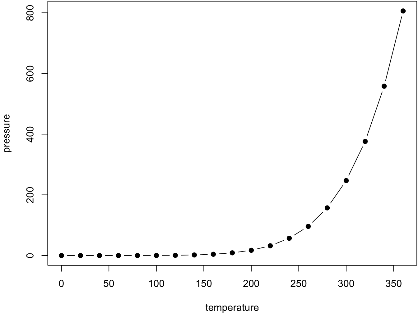
Figure 20.1: Here is a nice figure!
When you are writing code that generates images, and will produce images that will stay in your folders, make sure it is written to the img/ folder or a subfolder.
Here is an example of a table generated by R from a code chunk:
Don't miss Table \@ref(tab:nice-tab).

```{r nice-tab, tidy=FALSE}
knitr::kable(
  head(pressure, 10), caption = 'Here is a nice table!',
  booktabs = TRUE
)
```
This renders into:
Don’t miss Table 20.1.
| temperature | pressure |
|---|---|
| 0 | 0.0002 |
| 20 | 0.0012 |
| 40 | 0.0060 |
| 60 | 0.0300 |
| 80 | 0.0900 |
| 100 | 0.2700 |
| 120 | 0.7500 |
| 140 | 1.8500 |
| 160 | 4.2000 |
| 180 | 8.8000 |
You can find more information on figures and tables in Bookdown here.